Rule 30: Difference between revisions
No edit summary |
No edit summary Tag: Manual revert |
||
| (18 intermediate revisions by the same user not shown) | |||
| Line 1: | Line 1: | ||
= Cellular Automaton Rule 30 Analysis = | = Cellular Automaton Rule 30 Analysis = | ||
== Rule Information == | |||
Rule Number: 30 Rule Class: III (Chaotic) Behavior: Chaotic, good random number generator | Rule Number: 30 | ||
Rule Class: III (Chaotic) | |||
Behavior: Chaotic, good random number generator | |||
=== Rule Pattern === | |||
Binary Rule Table: | Binary Rule Table: | ||
[[File:nb-1tdgck2pvdj5z.png|thumb|none|500px]] | |||
| | |||
| | |||
| | |||
Visual Rule Plot: | Visual Rule Plot: | ||
[[File:nb-1khcz9aluy6ac.png|thumb|none|500px]] | |||
=== Rule ArrayPlot === | |||
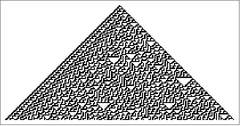
Canonical ArrayPlot: | Canonical ArrayPlot: | ||
[[File:nb-0riyiwjk34nk1.png|thumb|none|500px]] | |||
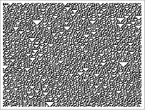
Random Initial Conditions ArrayPlot: | Random Initial Conditions ArrayPlot: | ||
[[File:nb-1ln8qo6u140ub.png|thumb|none|500px]] | |||
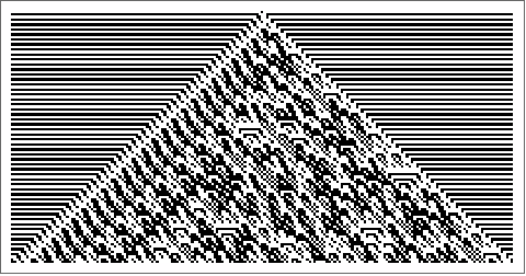
Alternate Step ArrayPlot: | Alternate Step ArrayPlot: | ||
[[File:nb-0c9h7u3akswvo.png|thumb|none|500px]] | |||
== Interactive Visualization == | |||
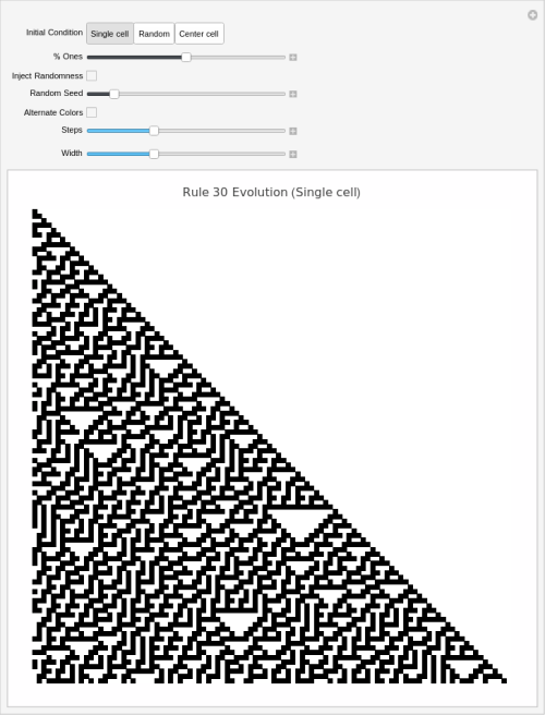
[[File:nb-17eddu8zr7uwf.png|thumb|none|500px]] | |||
== Continuously Injected Randomness Analysis == | |||
This shows 8 different trials of continuously injected randomness at the center position: | This shows 8 different trials of continuously injected randomness at the center position: | ||
[[File:nb-13ak18p4c0r5p.png|thumb|none|500px]] | |||
=== Understanding Randomness Injection === | |||
The 'Inject Randomness' feature transforms the cellular automaton from a deterministic system into a stochastic one by continuously adding random perturbations at the center position. This modification enables the study of several important phenomena: | |||
Robustness and Stability: How robust are the rule's patterns to constant disturbance? Some rules maintain their characteristic structures despite continuous noise, while others become completely randomized. This reveals the intrinsic stability of different cellular automaton classes. | |||
Pattern Propagation: Observe how random disturbances propagate through the system. Do they create expanding waves of disorder, or does the | Source Dynamics: The center position acts as a constant 'source' of randomness, simulating real-world systems where there's continuous environmental input or mutation. This is particularly relevant for modeling biological systems, chemical reactions, or social dynamics. | ||
Pattern Propagation: Observe how random disturbances propagate through the system. Do they create expanding waves of disorder, or does the rule's logic contain and process the randomness? Some rules can actually use randomness constructively to create more complex patterns. | |||
Noise Tolerance: Different rules show varying degrees of noise tolerance. Class I rules (uniform) may quickly absorb randomness, Class II rules (periodic) might maintain some structure, Class III rules (chaotic) may become even more random, while Class IV rules (complex) might show interesting noise-processing behaviors. | Noise Tolerance: Different rules show varying degrees of noise tolerance. Class I rules (uniform) may quickly absorb randomness, Class II rules (periodic) might maintain some structure, Class III rules (chaotic) may become even more random, while Class IV rules (complex) might show interesting noise-processing behaviors. | ||
| Line 82: | Line 57: | ||
Experimental Suggestions: Try comparing the same rule with and without randomness injection. Use different random seeds to see if patterns are consistent. Vary the initial conditions to see how randomness interacts with different starting configurations. | Experimental Suggestions: Try comparing the same rule with and without randomness injection. Use different random seeds to see if patterns are consistent. Vary the initial conditions to see how randomness interacts with different starting configurations. | ||
== Density Evolution == | |||
[[File:nb-14yhtky43h758.png|thumb|none|500px]] | |||
== Density Sensitivity Analysis == | |||
This shows how different random initial densities (5% to 95%) affect the rule's evolution: | |||
[[File:nb-0yoltszouo2sj.png|thumb|none|500px]] | |||
=== Understanding Density Effects === | |||
The density sensitivity analysis reveals how initial population density affects the | The density sensitivity analysis reveals how initial population density affects the rule's long-term behavior and pattern formation. This systematic comparison across different densities provides insights into several important aspects: | ||
Critical Thresholds: Many cellular automaton rules exhibit critical density thresholds where behavior changes dramatically. Below a certain density, patterns may die out or become sparse, while above it, rich structures emerge. This is analogous to phase transitions in physical systems like percolation or epidemic spread. | Critical Thresholds: Many cellular automaton rules exhibit critical density thresholds where behavior changes dramatically. Below a certain density, patterns may die out or become sparse, while above it, rich structures emerge. This is analogous to phase transitions in physical systems like percolation or epidemic spread. | ||
Density Independence vs. | Density Independence vs. Dependence: Some rules produce remarkably similar patterns regardless of initial density, suggesting robust underlying dynamics. Others show strong density dependence, where low densities create sparse, isolated structures while high densities produce dense, interacting patterns. | ||
Scale and Emergence: At larger scales ( | Scale and Emergence: At larger scales (100Ã100 cells), collective behaviors become visible that aren't apparent in smaller systems. Global patterns, waves, and large-scale structures can emerge from simple local rules, especially at intermediate densities where there's sufficient interaction without overcrowding. | ||
Population Dynamics Applications: This analysis is particularly relevant for modeling biological populations, where initial population density critically affects survival, growth patterns, and ecosystem stability. Different densities can represent different environmental conditions or initial colonization scenarios. | Population Dynamics Applications: This analysis is particularly relevant for modeling biological populations, where initial population density critically affects survival, growth patterns, and ecosystem stability. Different densities can represent different environmental conditions or initial colonization scenarios. | ||
Percolation and Connectivity: The density analysis helps identify percolation thresholds - the minimum density needed for patterns to | Percolation and Connectivity: The density analysis helps identify percolation thresholds - the minimum density needed for patterns to 'connect' across the entire space. This has applications in network theory, material science, and epidemic modeling. | ||
Research Applications: Use this analysis to identify interesting density ranges for further study, understand the | Research Applications: Use this analysis to identify interesting density ranges for further study, understand the rule's robustness to initial conditions, compare different rules' sensitivity to density, and validate theoretical predictions about critical phenomena in cellular automata. | ||
== Random Initial Condition Variability == | |||
This shows 8 different completely random initial conditions (50% density) to reveal variability in outcomes: | This shows 8 different completely random initial conditions (50% density) to reveal variability in outcomes: | ||
[[File:nb-0fitrx6r4dra7.png|thumb|none|500px]] | |||
=== Understanding Random Variability === | |||
The random initial condition variability analysis shows how the same rule behaves with different random starting configurations, all at approximately 50% density. This reveals the intrinsic variability and predictability of the | The random initial condition variability analysis shows how the same rule behaves with different random starting configurations, all at approximately 50% density. This reveals the intrinsic variability and predictability of the rule's dynamics: | ||
Deterministic vs. | Deterministic vs. Stochastic Appearance: Even though cellular automaton rules are completely deterministic, different random initial conditions can produce dramatically different outcomes. This analysis shows whether the rule tends toward similar final states regardless of starting configuration, or whether small differences in initial conditions lead to vastly different results. | ||
Pattern Consistency: Some rules produce remarkably consistent pattern types across all random initial conditions - similar textures, structures, or organizational principles emerge regardless of the specific starting arrangement. Others show high variability, with each evolution appearing almost unrelated to the others. | Pattern Consistency: Some rules produce remarkably consistent pattern types across all random initial conditions - similar textures, structures, or organizational principles emerge regardless of the specific starting arrangement. Others show high variability, with each evolution appearing almost unrelated to the others. | ||
| Line 129: | Line 101: | ||
Ergodic Properties: Rules that produce similar statistical properties (like final density, pattern frequency, or structural measures) across different random starts may have ergodic properties, where long-term averages are independent of initial conditions. | Ergodic Properties: Rules that produce similar statistical properties (like final density, pattern frequency, or structural measures) across different random starts may have ergodic properties, where long-term averages are independent of initial conditions. | ||
Practical Modeling Implications: In real-world applications, initial conditions are rarely known precisely. This analysis shows how robust the | Practical Modeling Implications: In real-world applications, initial conditions are rarely known precisely. This analysis shows how robust the rule's predictions are to uncertainty in initial states - crucial for modeling natural systems where exact initial configurations are impossible to determine. | ||
Statistical Analysis Opportunities: Use this set of evolutions to calculate statistical measures like final density distributions, pattern correlation lengths, or emergence times for specific structures. This provides quantitative characterization of the | Statistical Analysis Opportunities: Use this set of evolutions to calculate statistical measures like final density distributions, pattern correlation lengths, or emergence times for specific structures. This provides quantitative characterization of the rule's behavior under random initial conditions. | ||
== Damage Spreading Analysis == | |||
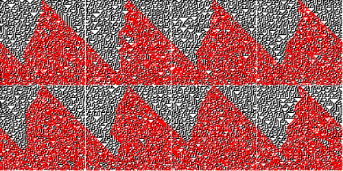
This shows how tiny perturbations (flipping one bit) propagate through the system. Red areas show where the perturbed and original evolutions differ: | This shows how tiny perturbations (flipping one bit) propagate through the system. Red areas show where the perturbed and original evolutions differ: | ||
[[File:nb-0durgt8omchk4.png|thumb|none|500px]] | |||
=== Understanding Damage Spreading === | |||
Damage spreading analysis reveals how cellular automaton rules respond to tiny perturbations - one of the most fundamental characteristics for understanding system stability and information propagation. This analysis starts with pairs of nearly identical initial conditions (differing by just one flipped bit) and tracks how this microscopic difference evolves: | Damage spreading analysis reveals how cellular automaton rules respond to tiny perturbations - one of the most fundamental characteristics for understanding system stability and information propagation. This analysis starts with pairs of nearly identical initial conditions (differing by just one flipped bit) and tracks how this microscopic difference evolves: | ||
Stability vs. | Stability vs. Sensitivity: Rules that quickly heal small perturbations (red areas disappear) demonstrate self-repair and stability properties. Those where tiny changes explode into large differences exhibit sensitive dependence on initial conditions - a hallmark of chaotic dynamics. This distinction is crucial for applications requiring robust, predictable behavior. | ||
Information Propagation: The red difference regions show exactly how information travels through the cellular automaton. Some rules propagate changes in expanding cones at specific speeds, others create complex interference patterns, and some maintain localized damage that neither grows nor shrinks. | Information Propagation: The red difference regions show exactly how information travels through the cellular automaton. Some rules propagate changes in expanding cones at specific speeds, others create complex interference patterns, and some maintain localized damage that neither grows nor shrinks. | ||
| Line 162: | Line 129: | ||
Research Opportunities: Use damage spreading patterns to classify rules, measure information propagation speeds, identify critical parameters, study phase transitions, and validate theoretical predictions about complex system behavior. | Research Opportunities: Use damage spreading patterns to classify rules, measure information propagation speeds, identify critical parameters, study phase transitions, and validate theoretical predictions about complex system behavior. | ||
== Damage Spreading Dynamics == | |||
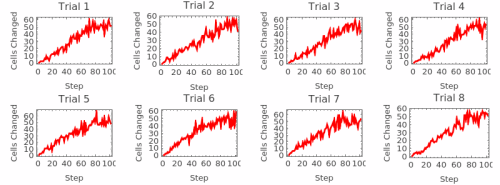
This shows the quantitative dynamics of damage spreading - how the number of differing cells changes over time: | This shows the quantitative dynamics of damage spreading - how the number of differing cells changes over time: | ||
[[File:nb-0ziw2kinh45cf.png|thumb|none|500px]] | |||
=== Understanding Damage Dynamics === | |||
The damage spreading dynamics plots provide quantitative time series data showing exactly how perturbations evolve numerically. Each graph tracks the number of cells that differ between the original and perturbed evolutions at every time step, revealing the mathematical structure underlying the visual patterns: | The damage spreading dynamics plots provide quantitative time series data showing exactly how perturbations evolve numerically. Each graph tracks the number of cells that differ between the original and perturbed evolutions at every time step, revealing the mathematical structure underlying the visual patterns: | ||
Growth vs. | Growth vs. Decay Patterns: The time series immediately reveal whether damage grows exponentially (indicating chaos), decays to zero (indicating stability), oscillates periodically (indicating cyclic repair), or reaches a steady state (indicating equilibrium between creation and annihilation of differences). | ||
Quantitative Classification: Different rule classes show characteristic damage dynamics signatures. Class I rules typically show rapid decay to zero, Class II rules often show oscillatory patterns, Class III rules frequently exhibit sustained growth or high-level fluctuations, while Class IV rules may show complex, intermediate behaviors. | Quantitative Classification: Different rule classes show characteristic damage dynamics signatures. Class I rules typically show rapid decay to zero, Class II rules often show oscillatory patterns, Class III rules frequently exhibit sustained growth or high-level fluctuations, while Class IV rules may show complex, intermediate behaviors. | ||
| Line 191: | Line 153: | ||
Practical Implications: For applications requiring predictable behavior, rules with rapidly decaying damage are preferred. For applications requiring sensitivity (like random number generation or mixing), rules with growing or sustained damage are valuable. For complex computation, rules showing intermediate damage dynamics often provide the best balance. | Practical Implications: For applications requiring predictable behavior, rules with rapidly decaying damage are preferred. For applications requiring sensitivity (like random number generation or mixing), rules with growing or sustained damage are valuable. For complex computation, rules showing intermediate damage dynamics often provide the best balance. | ||
== Damage Spreading Width Analysis == | |||
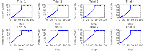
This measures the spatial extent (light cone) of damage spreading - how wide the perturbation influence spreads over time: | This measures the spatial extent (light cone) of damage spreading - how wide the perturbation influence spreads over time: | ||
[[File:nb-1h6b9rwbnvfeg.png|thumb|none|500px]] | |||
=== Understanding Spatial Propagation === | |||
The damage spreading width analysis measures the spatial extent of perturbation influence over time, revealing fundamental properties of information propagation and the cellular automaton's 'light cone' structure. This analysis tracks how far the effects of a single bit flip spread spatially as the system evolves: | |||
The damage spreading width analysis measures the spatial extent of perturbation influence over time, revealing fundamental properties of information propagation and the cellular | |||
Information Propagation Speed: The slope of the width curve reveals the maximum speed at which information can travel through the cellular automaton. Linear growth indicates constant propagation speed, while curved growth suggests acceleration, deceleration, or complex propagation dynamics. Many elementary rules show characteristic maximum speeds (often 1 cell per time step). | Information Propagation Speed: The slope of the width curve reveals the maximum speed at which information can travel through the cellular automaton. Linear growth indicates constant propagation speed, while curved growth suggests acceleration, deceleration, or complex propagation dynamics. Many elementary rules show characteristic maximum speeds (often 1 cell per time step). | ||
Light Cone Structure: In physics, a light cone defines the region of spacetime that can be influenced by an event. Similarly, this analysis reveals the cellular | Light Cone Structure: In physics, a light cone defines the region of spacetime that can be influenced by an event. Similarly, this analysis reveals the cellular automaton's causal structure - how far influence can reach in a given time. This is fundamental for understanding locality and information processing capabilities. | ||
Ballistic vs. | Ballistic vs. Diffusive Spreading: Linear width growth indicates ballistic propagation (like particles moving at constant speed), while square-root growth suggests diffusive spreading (like random walk processes). Some rules show intermediate behaviors or transitions between regimes, indicating complex underlying dynamics. | ||
Finite-Size Effects: When the damage width approaches the system size, boundary effects become important. The analysis reveals whether damage reflects off boundaries, wraps around (for periodic boundaries), or gets absorbed, providing insights into the | Finite-Size Effects: When the damage width approaches the system size, boundary effects become important. The analysis reveals whether damage reflects off boundaries, wraps around (for periodic boundaries), or gets absorbed, providing insights into the rule's behavior in finite systems. | ||
Stability Boundaries: The width analysis can reveal spatial stability boundaries - regions beyond which perturbations cannot propagate. Rules with bounded spreading show localization properties, while unbounded spreading indicates long-range correlation and potential for global influence from local changes. | Stability Boundaries: The width analysis can reveal spatial stability boundaries - regions beyond which perturbations cannot propagate. Rules with bounded spreading show localization properties, while unbounded spreading indicates long-range correlation and potential for global influence from local changes. | ||
| Line 222: | Line 179: | ||
Critical Behavior: Near critical points, width spreading often shows scale-invariant or power-law behavior. This can identify rules at phase transition boundaries where small parameter changes lead to qualitatively different spatial propagation properties. | Critical Behavior: Near critical points, width spreading often shows scale-invariant or power-law behavior. This can identify rules at phase transition boundaries where small parameter changes lead to qualitatively different spatial propagation properties. | ||
== Ensemble Properties == | |||
These analyses examine statistical properties averaged over many random initial conditions, revealing the rule's fundamental characteristics beyond individual evolutions: | |||
=== Power Spectrum Analysis === | |||
[[File:nb-08adkesvivofk.png|thumb|none|500px]] | |||
=== Ensemble Density Evolution === | |||
1. Enhanced Density Evolution Heatmap: | |||
[[File:nb-1m81codpqxt2u.png|thumb|none|500px]] | |||
2. Density Contour Plot: | |||
[[File:nb- | [[File:nb-1ai0nbdy8qj7r.png|thumb|none|500px]] | ||
3. Individual Density Trajectories: | |||
[[File:nb-1mx1gymcg3npb.png|thumb|none|500px]] | |||
4. Statistical Summary: | |||
[[File:nb-0e29sdvzf60z6.png|thumb|none|500px]] | |||
5. Final State Distribution: | |||
[[File:nb- | [[File:nb-05h8mckmbo1yb.png|thumb|none|500px]] | ||
=== Understanding Ensemble Properties === | |||
Ensemble properties reveal the | Ensemble properties reveal the rule's fundamental statistical behavior by averaging over many random initial conditions, providing insights that single evolutions cannot capture. These analyses are essential for understanding the cellular automaton's intrinsic characteristics: | ||
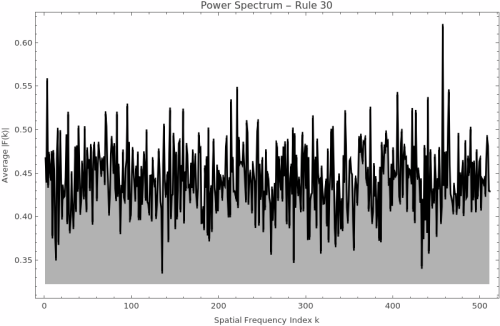
Power Spectrum Insights: The power spectrum measures the frequencies of spatial patterns in the final evolved state, revealing the | Power Spectrum Insights: The power spectrum measures the frequencies of spatial patterns in the final evolved state, revealing the rule's preference for certain spatial scales. A flat spectrum suggests random-like activity with no preferred frequencies, while peaks indicate characteristic wavelengths or periodic structures. Sharp peaks suggest regular patterns, while broad peaks indicate quasi-periodic or complex spatial organization. | ||
Density Evolution Dynamics: The density evolution heatmap | Density Evolution Dynamics: The density evolution heatmap Ï(p,t) shows how density changes over time for ALL possible initial densities simultaneously. Horizontal patterns indicate conservation (density preserved), upward trends show growth dynamics, downward trends indicate decay, and complex curves reveal non-trivial population dynamics. This comprehensive view reveals phase transitions and critical densities. | ||
Conservation vs. | Conservation vs. Growth Patterns: Horizontal lines in the density evolution indicate conservative rules that maintain density over time. Upward or downward trends show rules that systematically create or destroy cells. Complex curves indicate rules with intricate population dynamics that depend on both initial density and time. | ||
Attractor Analysis: The final density distribution | Attractor Analysis: The final density distribution Ï_final(p) reveals the rule's long-term attractors. A diagonal line indicates identity mapping (final density equals initial density), horizontal lines show fixed-point attractors regardless of initial conditions, and complex curves indicate multiple attractors or chaotic behavior with sensitive dependence on initial density. | ||
Critical Phenomena Detection: Sharp transitions in the density evolution heatmap often indicate critical phenomena and phase boundaries. These appear as sudden changes in behavior at specific initial densities, revealing critical thresholds where the | Critical Phenomena Detection: Sharp transitions in the density evolution heatmap often indicate critical phenomena and phase boundaries. These appear as sudden changes in behavior at specific initial densities, revealing critical thresholds where the rule's qualitative behavior changes dramatically. | ||
Sensitivity Assessment: Smooth gradients in the heatmap indicate robust behavior where small changes in initial density lead to small changes in evolution. Sharp boundaries or chaotic patterns reveal sensitive dependence on initial conditions - the hallmark of chaotic dynamics. | Sensitivity Assessment: Smooth gradients in the heatmap indicate robust behavior where small changes in initial density lead to small changes in evolution. Sharp boundaries or chaotic patterns reveal sensitive dependence on initial conditions - the hallmark of chaotic dynamics. | ||
| Line 298: | Line 229: | ||
Research Applications: Use density evolution analysis to classify rules by their population dynamics, identify critical densities and phase transitions, predict long-term behavior from initial conditions, compare different rules quantitatively, and validate theoretical predictions about cellular automaton attractors and conservation laws. | Research Applications: Use density evolution analysis to classify rules by their population dynamics, identify critical densities and phase transitions, predict long-term behavior from initial conditions, compare different rules quantitatively, and validate theoretical predictions about cellular automaton attractors and conservation laws. | ||
== Finite Size Properties == | |||
These analyses examine the rule's behavior in small, finite systems, revealing attractor structure and repetition periods. State Transition Diagrams are directed graphs, where each node represents a possible binary configuration of the grid (with periodic boundaries). An arrow connects one state to its successor, given the automaton's rule. Loops and cycles correspond to repeating patternsâattractors in the finite CA. How Would You Construct One by Hand? Choose a grid width (e.g., 3 cells). List all possible states. For 3 cells: 000, 001, 010, 011, 100, 101, 110, 111. For each state: Apply the CA rule (with periodic boundaries) to generate the next state. Cells update according to the values of themselves and their left/right neighbors (use the rule's lookup table). Draw an arrow from the current state to its next state. Repeat until every state is mapped. Visualize the graph: Arrange nodes so cycles (loops) and branches are clear. | |||
=== State Transition Diagrams === | |||
[[File:nb- | [[File:nb-0ime33tbv9yyk.png|thumb|none|500px]] | ||
=== Understanding State Transition Diagrams === | |||
State transition diagrams provide a complete map of the cellular | State transition diagrams provide a complete map of the cellular automaton's behavior in finite systems, showing every possible configuration and how it evolves. Each node represents a unique binary configuration of the grid (with periodic boundaries), and directed edges show which state follows which under one application of the rule. | ||
Reading the Graphs: In these directed graphs, nodes are numbered 0 to 2^n-1, representing all possible binary strings of length n. | Reading the Graphs: In these directed graphs, nodes are numbered 0 to 2^n-1, representing all possible binary strings of length n. An arrow from node A to node B means configuration A evolves to configuration B in one time step. Loops (cycles) indicate repeating patterns - attractors the system settles into. Trees branching into loops show transient states that eventually reach attractors but aren't part of the cycle themselves. | ||
Manual Construction: To construct a state transition diagram by hand: (1) Choose a grid width (e.g., 3 cells). (2) List all possible states (for 3 cells: 000, 001, 010, 011, 100, 101, 110, 111). (3) For each state, apply the CA rule with periodic boundaries - each cell updates based on itself and its left/right neighbors using the | Manual Construction: To construct a state transition diagram by hand: (1) Choose a grid width (e.g., 3 cells). (2) List all possible states (for 3 cells: 000, 001, 010, 011, 100, 101, 110, 111). (3) For each state, apply the CA rule with periodic boundaries - each cell updates based on itself and its left/right neighbors using the rule's lookup table. (4) Draw an arrow from each current state to its successor. (5) Arrange nodes so cycles and branches are visually clear. | ||
Attractor Topology: The graph structure immediately reveals the | Attractor Topology: The graph structure immediately reveals the rule's attractor landscape. Fixed points appear as self-loops (nodes with arrows to themselves). Periodic orbits appear as polygons - triangles for period-3, squares for period-4, etc. Complex rules show intricate branching structures with multiple separate attractor basins, while simple rules often collapse to one or two fixed points. | ||
Transient vs. | Transient vs. Recurrent States: States on cycles are recurrent - the system returns to them infinitely often. States not on cycles are transient - visited at most once before reaching an attractor. The ratio of transient to recurrent states indicates how much 'memory' the rule has about initial conditions versus how quickly it forgets and settles into repetitive behavior. | ||
Reversibility Detection: A reversible rule has every node with exactly one incoming edge - each state has exactly one predecessor. This creates a graph of pure cycles with no trees. Non-reversible rules have states with multiple predecessors (many-to-one mapping) and states with no predecessors (Garden of Eden configurations). The visual topology immediately reveals reversibility. | Reversibility Detection: A reversible rule has every node with exactly one incoming edge - each state has exactly one predecessor. This creates a graph of pure cycles with no trees. Non-reversible rules have states with multiple predecessors (many-to-one mapping) and states with no predecessors (Garden of Eden configurations). The visual topology immediately reveals reversibility. | ||
| Line 330: | Line 255: | ||
Connectivity and Components: The number of disconnected components (separate subgraphs) reveals how many independent attractor basins exist. A single component means all initial conditions eventually interact or merge into one attractor system. Multiple components indicate the rule partitions state space into isolated dynamical subsystems that never influence each other. | Connectivity and Components: The number of disconnected components (separate subgraphs) reveals how many independent attractor basins exist. A single component means all initial conditions eventually interact or merge into one attractor system. Multiple components indicate the rule partitions state space into isolated dynamical subsystems that never influence each other. | ||
Cycle Lengths and Periods: The perimeter of each polygon gives the cycle length. Count the nodes in a loop to determine the period. The longest cycle in the graph is the maximum repetition period for that system size. Comparing maximum cycle lengths across different widths reveals how the | Cycle Lengths and Periods: The perimeter of each polygon gives the cycle length. Count the nodes in a loop to determine the period. The longest cycle in the graph is the maximum repetition period for that system size. Comparing maximum cycle lengths across different widths reveals how the rule's temporal complexity scales with spatial size. | ||
Symmetry and Structure: Look for symmetries in the graph layout - they often reflect symmetries in the rule itself (left-right symmetry, complement symmetry, etc.). Highly regular, symmetric graphs suggest simple, structured rules. Asymmetric, irregular graphs indicate complex, less predictable behavior. | Symmetry and Structure: Look for symmetries in the graph layout - they often reflect symmetries in the rule itself (left-right symmetry, complement symmetry, etc.). Highly regular, symmetric graphs suggest simple, structured rules. Asymmetric, irregular graphs indicate complex, less predictable behavior. | ||
| Line 338: | Line 263: | ||
Research Applications: Use state transition diagrams to classify rules by attractor topology, identify reversible rules visually, count Garden of Eden states, measure basin sizes for different attractors, validate theoretical predictions about finite CA behavior, and understand the complete finite-state dynamics that infinite systems approximate. | Research Applications: Use state transition diagrams to classify rules by attractor topology, identify reversible rules visually, count Garden of Eden states, measure basin sizes for different attractors, validate theoretical predictions about finite CA behavior, and understand the complete finite-state dynamics that infinite systems approximate. | ||
=== Maximum Cycle Length Analysis === | |||
[[File:nb-112vziins32fs.png|thumb|none|500px]] | |||
=== Understanding Cycle Length and Finite Size Properties === | |||
Finite size analysis reveals the rule's fundamental mathematical structure by examining complete state spaces in small systems. Since every finite CA must eventually return to a previously visited state, all trajectories lead to attractors - either fixed points (cycle length 1) or periodic cycles. The maximum cycle length provides a measure of the rule's dynamical complexity and computational depth in finite systems. | |||
State Transition Structure: The directed graphs show every possible state and its successor, revealing the rule's complete attractor structure. Cycles appear as polygons (closed loops), while transient states form trees leading to attractors. This topology reveals whether the rule has simple fixed points, complex cycles, or chaotic attractors in finite systems. | |||
Theoretical Maximum and Complexity Bounds: In a system with n cells, there are exactly 2^n possible configurations, providing an absolute upper bound on cycle length. Rules approaching this maximum exhibit highly complex, pseudo-chaotic behavior where the system takes exponentially long to repeat. The ratio of actual maximum cycle to theoretical maximum quantifies the rule's effective state space utilization. | |||
Theoretical Maximum and Complexity Bounds: In a system with n cells, there are exactly 2^n possible configurations, providing an absolute upper bound on cycle length. Rules approaching this maximum exhibit highly complex, pseudo-chaotic behavior where the system takes exponentially long to repeat. The ratio of actual maximum cycle to theoretical maximum quantifies the | |||
Exponential vs Polynomial Growth: Different rule classes show characteristic scaling behaviors. Class I rules typically maintain cycle length 1 across all system sizes. Class II rules often show small constant or slowly growing cycle lengths. Class III rules may show exponential growth approaching theoretical limits, while Class IV rules can exhibit intermediate polynomial growth patterns. | Exponential vs Polynomial Growth: Different rule classes show characteristic scaling behaviors. Class I rules typically maintain cycle length 1 across all system sizes. Class II rules often show small constant or slowly growing cycle lengths. Class III rules may show exponential growth approaching theoretical limits, while Class IV rules can exhibit intermediate polynomial growth patterns. | ||
| Line 365: | Line 285: | ||
Practical Applications: For cryptography, rules with exponentially growing cycles are desirable. For modeling periodic phenomena, rules with predictable small cycles are useful. For random number generation, rules with maximal cycles provide good pseudo-randomness with known periodicity. | Practical Applications: For cryptography, rules with exponentially growing cycles are desirable. For modeling periodic phenomena, rules with predictable small cycles are useful. For random number generation, rules with maximal cycles provide good pseudo-randomness with known periodicity. | ||
=== Backtracking Trees === | |||
This shows the tree of all possible predecessor configurations that can produce a given target pattern, revealing the | This shows the tree of all possible predecessor configurations that can produce a given target pattern, revealing the rule's preimage structure: | ||
[[File:nb-0arj4jfal7gqq.png|thumb|none|500px]] | |||
[[File:nb- | [[File:nb-0sckwx13dw072.png|thumb|none|500px]] | ||
=== Understanding Backtracking Trees === | |||
Backtracking trees reveal the inverse dynamics of cellular automata by showing all possible configurations that could have produced a given target pattern. Unlike forward evolution which is deterministic (one input produces one output), backward evolution is typically non-deterministic - multiple different predecessors can produce the same successor configuration. | Backtracking trees reveal the inverse dynamics of cellular automata by showing all possible configurations that could have produced a given target pattern. Unlike forward evolution which is deterministic (one input produces one output), backward evolution is typically non-deterministic - multiple different predecessors can produce the same successor configuration. | ||
Reading the Tree Structure: The root node (top or center) shows the target configuration | Reading the Tree Structure: The root node (top or center) shows the target configuration you're working backward from. Each branch downward represents one time step backward in evolution. At each level, nodes show all possible predecessor configurations. The branching factor indicates how many different ways that configuration could have been produced. Dead ends (leaves) occur when no valid predecessors exist. | ||
Surjectivity and Preimage Structure: The tree immediately reveals whether the rule is surjective (onto). If every possible configuration appears somewhere in the tree when run long enough, the rule is surjective - all configurations are reachable. Configurations that never appear are Garden of Eden states - they have no predecessors and can only exist as initial conditions, never arising from evolution. | Surjectivity and Preimage Structure: The tree immediately reveals whether the rule is surjective (onto). If every possible configuration appears somewhere in the tree when run long enough, the rule is surjective - all configurations are reachable. Configurations that never appear are Garden of Eden states - they have no predecessors and can only exist as initial conditions, never arising from evolution. | ||
| Line 397: | Line 303: | ||
Reversibility Detection: A reversible rule produces trees where every node has exactly one child at each level - no branching, just a single path backward. This one-to-one correspondence between successors and predecessors defines reversibility. Non-reversible rules show branching (many-to-one mapping) or dead ends (states with no predecessors). | Reversibility Detection: A reversible rule produces trees where every node has exactly one child at each level - no branching, just a single path backward. This one-to-one correspondence between successors and predecessors defines reversibility. Non-reversible rules show branching (many-to-one mapping) or dead ends (states with no predecessors). | ||
Expansion vs. | Expansion vs. Contraction: Watch how the tree grows or shrinks with depth. Expanding trees (branching factor > 1) indicate many configurations map to few - information is being compressed in forward evolution. Contracting trees suggest divergent forward dynamics. Balanced trees indicate conservation of information. The average branching factor quantifies this expansion/contraction rate. | ||
Computational Complexity: The | Computational Complexity: The tree's size and structure reveal computational properties. Exponentially growing trees indicate the rule is computationally complex backward - finding predecessors is hard even if forward evolution is simple. Small, finite trees suggest limited backward complexity. The tree's depth and breadth relate to the rule's descriptive complexity. | ||
Pattern Propagation Backward: The tree shows how localized patterns in the target decompose into potentially more complex predecessor patterns. Some rules maintain locality (local patterns have local predecessors), while others show that simple local patterns require complex non-local predecessor arrangements. This reveals the | Pattern Propagation Backward: The tree shows how localized patterns in the target decompose into potentially more complex predecessor patterns. Some rules maintain locality (local patterns have local predecessors), while others show that simple local patterns require complex non-local predecessor arrangements. This reveals the rule's information structure. | ||
Symmetry and Structure: Look for symmetries in the tree - they reflect symmetries in the rule itself. Symmetric trees suggest the rule treats space uniformly. Asymmetric trees may indicate directional bias or broken symmetries. Regular, repetitive tree structure indicates predictable preimage patterns. | Symmetry and Structure: Look for symmetries in the tree - they reflect symmetries in the rule itself. Symmetric trees suggest the rule treats space uniformly. Asymmetric trees may indicate directional bias or broken symmetries. Regular, repetitive tree structure indicates predictable preimage patterns. | ||
| Line 417: | Line 323: | ||
Research Applications: Use backtracking trees to classify rules by preimage structure, identify Garden of Eden states, measure surjectivity, detect reversibility, quantify information loss in forward evolution, understand pattern formation constraints, and study the inverse problem of cellular automaton dynamics. | Research Applications: Use backtracking trees to classify rules by preimage structure, identify Garden of Eden states, measure surjectivity, detect reversibility, quantify information loss in forward evolution, understand pattern formation constraints, and study the inverse problem of cellular automaton dynamics. | ||
== State Space as Cantor Set == | |||
The CA rule as a continuous mapping on [0,1]. Each point represents a binary configuration normalized to the unit interval: | The CA rule as a continuous mapping on [0,1]. Each point represents a binary configuration normalized to the unit interval: | ||
=== Cantor Set Mapping === | |||
[[File:nb-0uge3ls882wni.png|thumb|none|500px]] | |||
=== High Resolution View === | |||
[[File:nb- | [[File:nb-1x337oyxa2muh.png|thumb|none|500px]] | ||
=== Understanding the Cantor Set Representation === | |||
The Cantor set visualization reveals one of the most profound connections between cellular automata and pure mathematics, showing how discrete, local rules generate continuous dynamical systems with rich topological structure. This representation transforms our understanding of CAs from computational objects to mathematical functions with deep geometric properties: | The Cantor set visualization reveals one of the most profound connections between cellular automata and pure mathematics, showing how discrete, local rules generate continuous dynamical systems with rich topological structure. This representation transforms our understanding of CAs from computational objects to mathematical functions with deep geometric properties: | ||
Mathematical Foundation and Construction: Each configuration of n cells can be uniquely encoded as a binary number between 0 and 2^n-1. Dividing by 2^n maps this integer to a point in [0,1]. For example, with n=3, the configuration 101 becomes 5/8 = 0.625. The CA rule then defines a function f:[0,1] | Mathematical Foundation and Construction: Each configuration of n cells can be uniquely encoded as a binary number between 0 and 2^n-1. Dividing by 2^n maps this integer to a point in [0,1]. For example, with n=3, the configuration 101 becomes 5/8 = 0.625. The CA rule then defines a function f:[0,1]â[0,1] where f maps each normalized configuration to its successor. As nââ, the domain converges to a Cantor set - a perfect, nowhere dense, uncountable fractal subset of [0,1] with total length zero but cardinality 2^âµâ. | ||
Continuity from Locality: The CA | Continuity from Locality: The CA rule's locality (each cell depends only on its neighborhood) directly implies the function's continuity. Configurations differing by a single bit in position i differ by approximately 1/2^i in the normalized representation. Since the rule's output at any position depends only on nearby bits, small changes in input produce small changes in output. This topological property connects discrete computation to continuous dynamics. | ||
Fractal Self-Similarity and Scaling: The self-similar patterns visible in the plot reflect the | Fractal Self-Similarity and Scaling: The self-similar patterns visible in the plot reflect the rule's shift-invariance and local nature. When you zoom into any region, you see similar structures at finer scales. This isn't just visual aesthetics - it's a fundamental property of the mapping. The fractal dimension of the graph can characterize the rule's complexity, with simple rules producing low-dimensional graphs and complex rules generating space-filling or high-dimensional structures. | ||
Fixed Points and Diagonal Structure: Points on the diagonal y=x represent configurations that | Fixed Points and Diagonal Structure: Points on the diagonal y=x represent configurations that don't change under one application of the rule - fixed points in the dynamical system. Periodic orbits appear as discrete sets of points that cycle through each other. The distance from the diagonal indicates how dramatically the rule transforms each configuration. Rules hugging the diagonal are nearly identity functions, while those with large deviations show strong transformative behavior. | ||
Surjectivity and Image Structure: A surjective (onto) rule produces a graph that covers the full unit square, meaning every configuration is reachable from some predecessor. Gaps in the vertical direction reveal non-surjectivity - certain configurations (Garden of Eden states) have no predecessors. The distribution of these gaps provides deep information about the | Surjectivity and Image Structure: A surjective (onto) rule produces a graph that covers the full unit square, meaning every configuration is reachable from some predecessor. Gaps in the vertical direction reveal non-surjectivity - certain configurations (Garden of Eden states) have no predecessors. The distribution of these gaps provides deep information about the rule's information-theoretic properties and entropy production. | ||
Symbolic Dynamics Connection: This representation directly connects CAs to symbolic dynamics, a branch of dynamical systems theory studying shift spaces. The shift map (moving a configuration one position) becomes conjugate to a topological operation on the Cantor set. Properties like mixing, minimality, and topological entropy have precise meanings in this framework, allowing rigorous analysis of CA behavior using powerful mathematical tools. | Symbolic Dynamics Connection: This representation directly connects CAs to symbolic dynamics, a branch of dynamical systems theory studying shift spaces. The shift map (moving a configuration one position) becomes conjugate to a topological operation on the Cantor set. Properties like mixing, minimality, and topological entropy have precise meanings in this framework, allowing rigorous analysis of CA behavior using powerful mathematical tools. | ||
| Line 457: | Line 353: | ||
Chaos and Sensitivity: In this representation, chaotic behavior manifests as sensitive dependence on initial conditions - nearby input points can map to distant output points. The Lyapunov exponent, measuring exponential separation of trajectories, can be visualized through the local slope of the mapping. Class III rules typically show highly irregular, space-filling graphs indicating chaotic dynamics, while Class I rules produce simple, structured graphs. | Chaos and Sensitivity: In this representation, chaotic behavior manifests as sensitive dependence on initial conditions - nearby input points can map to distant output points. The Lyapunov exponent, measuring exponential separation of trajectories, can be visualized through the local slope of the mapping. Class III rules typically show highly irregular, space-filling graphs indicating chaotic dynamics, while Class I rules produce simple, structured graphs. | ||
Measure Theory and Invariant Measures: For many CA rules, there exists an invariant measure on the Cantor set - a probability distribution preserved by the | Measure Theory and Invariant Measures: For many CA rules, there exists an invariant measure on the Cantor set - a probability distribution preserved by the rule's action. The density of points in different regions of the plot hints at this measure. Rules preserving Bernoulli measure (uniform density) appear as evenly distributed points, while those with non-trivial invariant measures show clustering in specific regions. This connects to ergodic theory and statistical mechanics. | ||
Reversibility and Bijection: Reversible CA rules produce bijective (one-to-one and onto) functions on the Cantor set. In the plot, this appears as a graph where each horizontal line intersects exactly once - every output has exactly one input. The graph of a reversible rule has special symmetry properties and preserves measure, making it a measure-preserving transformation of fundamental importance in ergodic theory. | Reversibility and Bijection: Reversible CA rules produce bijective (one-to-one and onto) functions on the Cantor set. In the plot, this appears as a graph where each horizontal line intersects exactly once - every output has exactly one input. The graph of a reversible rule has special symmetry properties and preserves measure, making it a measure-preserving transformation of fundamental importance in ergodic theory. | ||
Computational Complexity from Geometry: The geometric complexity of the Cantor set graph correlates with computational complexity. Simple rules produce smooth or piecewise-linear graphs, while computationally universal rules (like Rule 110) generate graphs with infinite complexity at all scales. The algorithmic information content of the | Computational Complexity from Geometry: The geometric complexity of the Cantor set graph correlates with computational complexity. Simple rules produce smooth or piecewise-linear graphs, while computationally universal rules (like Rule 110) generate graphs with infinite complexity at all scales. The algorithmic information content of the graph's description relates to the rule's computational power. | ||
Research Applications: Use the Cantor set representation to rigorously classify rules by topological properties, compute invariant measures and entropy rates, identify reversible rules through graph symmetry, study bifurcations and phase transitions, connect CA theory to broader dynamical systems theory, and visualize abstract properties like mixing and minimality. | Research Applications: Use the Cantor set representation to rigorously classify rules by topological properties, compute invariant measures and entropy rates, identify reversible rules through graph symmetry, study bifurcations and phase transitions, connect CA theory to broader dynamical systems theory, and visualize abstract properties like mixing and minimality. | ||
Latest revision as of 06:33, 18 November 2025
Cellular Automaton Rule 30 Analysis
Rule Information
Rule Number: 30 Rule Class: III (Chaotic) Behavior: Chaotic, good random number generator
Rule Pattern
Binary Rule Table:

Visual Rule Plot:

Rule ArrayPlot
Canonical ArrayPlot:
Random Initial Conditions ArrayPlot:
Alternate Step ArrayPlot:
Interactive Visualization
Continuously Injected Randomness Analysis
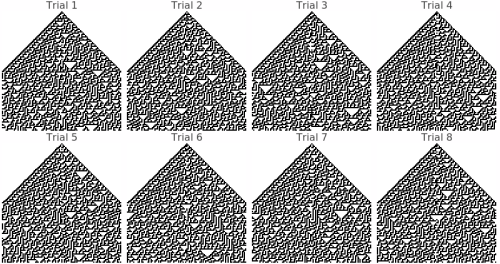
This shows 8 different trials of continuously injected randomness at the center position:
Understanding Randomness Injection
The 'Inject Randomness' feature transforms the cellular automaton from a deterministic system into a stochastic one by continuously adding random perturbations at the center position. This modification enables the study of several important phenomena:
Robustness and Stability: How robust are the rule's patterns to constant disturbance? Some rules maintain their characteristic structures despite continuous noise, while others become completely randomized. This reveals the intrinsic stability of different cellular automaton classes.
Source Dynamics: The center position acts as a constant 'source' of randomness, simulating real-world systems where there's continuous environmental input or mutation. This is particularly relevant for modeling biological systems, chemical reactions, or social dynamics.
Pattern Propagation: Observe how random disturbances propagate through the system. Do they create expanding waves of disorder, or does the rule's logic contain and process the randomness? Some rules can actually use randomness constructively to create more complex patterns.
Noise Tolerance: Different rules show varying degrees of noise tolerance. Class I rules (uniform) may quickly absorb randomness, Class II rules (periodic) might maintain some structure, Class III rules (chaotic) may become even more random, while Class IV rules (complex) might show interesting noise-processing behaviors.
Real-World Applications: This feature models systems like biological evolution with constant mutation, economic markets with random external shocks, information transmission through noisy channels, ecosystem dynamics with environmental perturbations, and neural networks with synaptic noise.
Experimental Suggestions: Try comparing the same rule with and without randomness injection. Use different random seeds to see if patterns are consistent. Vary the initial conditions to see how randomness interacts with different starting configurations.
Density Evolution
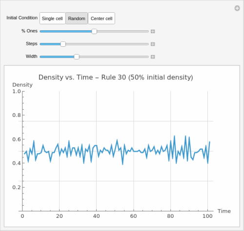
Density Sensitivity Analysis
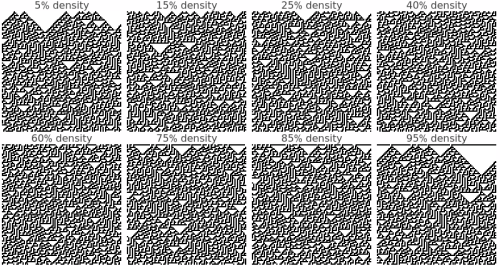
This shows how different random initial densities (5% to 95%) affect the rule's evolution:
Understanding Density Effects
The density sensitivity analysis reveals how initial population density affects the rule's long-term behavior and pattern formation. This systematic comparison across different densities provides insights into several important aspects:
Critical Thresholds: Many cellular automaton rules exhibit critical density thresholds where behavior changes dramatically. Below a certain density, patterns may die out or become sparse, while above it, rich structures emerge. This is analogous to phase transitions in physical systems like percolation or epidemic spread.
Density Independence vs. Dependence: Some rules produce remarkably similar patterns regardless of initial density, suggesting robust underlying dynamics. Others show strong density dependence, where low densities create sparse, isolated structures while high densities produce dense, interacting patterns.
Scale and Emergence: At larger scales (100Ã100 cells), collective behaviors become visible that aren't apparent in smaller systems. Global patterns, waves, and large-scale structures can emerge from simple local rules, especially at intermediate densities where there's sufficient interaction without overcrowding.
Population Dynamics Applications: This analysis is particularly relevant for modeling biological populations, where initial population density critically affects survival, growth patterns, and ecosystem stability. Different densities can represent different environmental conditions or initial colonization scenarios.
Percolation and Connectivity: The density analysis helps identify percolation thresholds - the minimum density needed for patterns to 'connect' across the entire space. This has applications in network theory, material science, and epidemic modeling.
Research Applications: Use this analysis to identify interesting density ranges for further study, understand the rule's robustness to initial conditions, compare different rules' sensitivity to density, and validate theoretical predictions about critical phenomena in cellular automata.
Random Initial Condition Variability
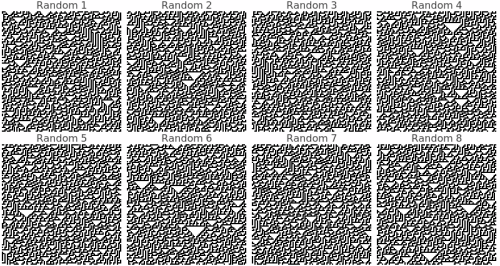
This shows 8 different completely random initial conditions (50% density) to reveal variability in outcomes:
Understanding Random Variability
The random initial condition variability analysis shows how the same rule behaves with different random starting configurations, all at approximately 50% density. This reveals the intrinsic variability and predictability of the rule's dynamics:
Deterministic vs. Stochastic Appearance: Even though cellular automaton rules are completely deterministic, different random initial conditions can produce dramatically different outcomes. This analysis shows whether the rule tends toward similar final states regardless of starting configuration, or whether small differences in initial conditions lead to vastly different results.
Pattern Consistency: Some rules produce remarkably consistent pattern types across all random initial conditions - similar textures, structures, or organizational principles emerge regardless of the specific starting arrangement. Others show high variability, with each evolution appearing almost unrelated to the others.
Sensitivity to Initial Conditions: This visualization reveals whether the rule exhibits sensitive dependence on initial conditions (a hallmark of chaotic systems). If tiny differences in initial random arrangements lead to completely different outcomes, this suggests chaotic dynamics.
Ergodic Properties: Rules that produce similar statistical properties (like final density, pattern frequency, or structural measures) across different random starts may have ergodic properties, where long-term averages are independent of initial conditions.
Practical Modeling Implications: In real-world applications, initial conditions are rarely known precisely. This analysis shows how robust the rule's predictions are to uncertainty in initial states - crucial for modeling natural systems where exact initial configurations are impossible to determine.
Statistical Analysis Opportunities: Use this set of evolutions to calculate statistical measures like final density distributions, pattern correlation lengths, or emergence times for specific structures. This provides quantitative characterization of the rule's behavior under random initial conditions.
Damage Spreading Analysis
This shows how tiny perturbations (flipping one bit) propagate through the system. Red areas show where the perturbed and original evolutions differ:
Understanding Damage Spreading
Damage spreading analysis reveals how cellular automaton rules respond to tiny perturbations - one of the most fundamental characteristics for understanding system stability and information propagation. This analysis starts with pairs of nearly identical initial conditions (differing by just one flipped bit) and tracks how this microscopic difference evolves:
Stability vs. Sensitivity: Rules that quickly heal small perturbations (red areas disappear) demonstrate self-repair and stability properties. Those where tiny changes explode into large differences exhibit sensitive dependence on initial conditions - a hallmark of chaotic dynamics. This distinction is crucial for applications requiring robust, predictable behavior.
Information Propagation: The red difference regions show exactly how information travels through the cellular automaton. Some rules propagate changes in expanding cones at specific speeds, others create complex interference patterns, and some maintain localized damage that neither grows nor shrinks.
Error Correction Properties: In computational applications, this analysis reveals whether the rule has inherent error-correction capabilities. Rules that spontaneously repair small errors are valuable for robust computation and reliable information storage, while those that amplify errors might be useful for mixing and randomization.
Pattern Interaction Dynamics: Damage spreading often reveals how different structures in the cellular automaton interact with each other. Differences may propagate differently through various pattern types, showing which structures are stable and which are fragile to perturbations.
Critical Phenomena: Many rules exhibit critical points where damage spreading behavior changes dramatically. Near these critical points, the system may show scale-invariant damage patterns, long-range correlations, or power-law distributions - signatures of complex systems at the edge of chaos.
Real-World Applications: This analysis is essential for modeling biological evolution (mutation effects), network resilience (single node failures), material science (crack propagation), and social systems (rumor spreading). Understanding how small changes cascade through complex systems is fundamental to many scientific disciplines.
Research Opportunities: Use damage spreading patterns to classify rules, measure information propagation speeds, identify critical parameters, study phase transitions, and validate theoretical predictions about complex system behavior.
Damage Spreading Dynamics
This shows the quantitative dynamics of damage spreading - how the number of differing cells changes over time:
Understanding Damage Dynamics
The damage spreading dynamics plots provide quantitative time series data showing exactly how perturbations evolve numerically. Each graph tracks the number of cells that differ between the original and perturbed evolutions at every time step, revealing the mathematical structure underlying the visual patterns:
Growth vs. Decay Patterns: The time series immediately reveal whether damage grows exponentially (indicating chaos), decays to zero (indicating stability), oscillates periodically (indicating cyclic repair), or reaches a steady state (indicating equilibrium between creation and annihilation of differences).
Quantitative Classification: Different rule classes show characteristic damage dynamics signatures. Class I rules typically show rapid decay to zero, Class II rules often show oscillatory patterns, Class III rules frequently exhibit sustained growth or high-level fluctuations, while Class IV rules may show complex, intermediate behaviors.
Critical Point Detection: Near critical phase transitions, damage dynamics often show power-law scaling, long-term correlations, or scale-invariant fluctuations. These mathematical signatures can identify rules operating at the edge of chaos - often the most computationally interesting and complex.
Statistical Analysis Opportunities: These time series enable rigorous statistical analysis including autocorrelation functions, power spectral density, fractal dimension calculations, and entropy measures. Such analyses can distinguish between truly random fluctuations and deterministic chaos.
Comparative Analysis: By examining multiple trials (different random initial conditions), you can assess the consistency of damage dynamics. Some rules show highly reproducible damage curves, while others exhibit high variability depending on the specific initial configuration.
Information Theory Applications: The number of differing cells provides a direct measure of information divergence between the two evolutions. This connects to fundamental concepts in information theory, thermodynamics, and the physics of computation.
Practical Implications: For applications requiring predictable behavior, rules with rapidly decaying damage are preferred. For applications requiring sensitivity (like random number generation or mixing), rules with growing or sustained damage are valuable. For complex computation, rules showing intermediate damage dynamics often provide the best balance.
Damage Spreading Width Analysis
This measures the spatial extent (light cone) of damage spreading - how wide the perturbation influence spreads over time:
Understanding Spatial Propagation
The damage spreading width analysis measures the spatial extent of perturbation influence over time, revealing fundamental properties of information propagation and the cellular automaton's 'light cone' structure. This analysis tracks how far the effects of a single bit flip spread spatially as the system evolves:
Information Propagation Speed: The slope of the width curve reveals the maximum speed at which information can travel through the cellular automaton. Linear growth indicates constant propagation speed, while curved growth suggests acceleration, deceleration, or complex propagation dynamics. Many elementary rules show characteristic maximum speeds (often 1 cell per time step).
Light Cone Structure: In physics, a light cone defines the region of spacetime that can be influenced by an event. Similarly, this analysis reveals the cellular automaton's causal structure - how far influence can reach in a given time. This is fundamental for understanding locality and information processing capabilities.
Ballistic vs. Diffusive Spreading: Linear width growth indicates ballistic propagation (like particles moving at constant speed), while square-root growth suggests diffusive spreading (like random walk processes). Some rules show intermediate behaviors or transitions between regimes, indicating complex underlying dynamics.
Finite-Size Effects: When the damage width approaches the system size, boundary effects become important. The analysis reveals whether damage reflects off boundaries, wraps around (for periodic boundaries), or gets absorbed, providing insights into the rule's behavior in finite systems.
Stability Boundaries: The width analysis can reveal spatial stability boundaries - regions beyond which perturbations cannot propagate. Rules with bounded spreading show localization properties, while unbounded spreading indicates long-range correlation and potential for global influence from local changes.
Computational Implications: For parallel computation applications, the width growth rate determines communication requirements and synchronization needs. Rules with bounded spreading can be computed efficiently in parallel, while those with rapid spreading require extensive inter-processor communication.
Pattern Formation Insights: The width dynamics reveal how local perturbations evolve into global patterns. Some rules show width oscillations indicating breathing patterns, others show plateaus suggesting stable structures, and some show complex width dynamics indicating intricate pattern interactions.
Critical Behavior: Near critical points, width spreading often shows scale-invariant or power-law behavior. This can identify rules at phase transition boundaries where small parameter changes lead to qualitatively different spatial propagation properties.
Ensemble Properties
These analyses examine statistical properties averaged over many random initial conditions, revealing the rule's fundamental characteristics beyond individual evolutions:
Power Spectrum Analysis
Ensemble Density Evolution
1. Enhanced Density Evolution Heatmap:
2. Density Contour Plot:
3. Individual Density Trajectories:
4. Statistical Summary:
5. Final State Distribution:
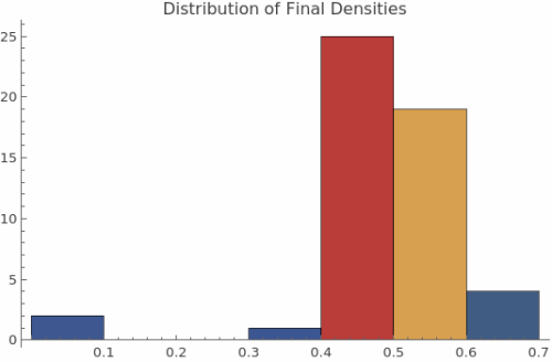
Understanding Ensemble Properties
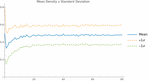
Ensemble properties reveal the rule's fundamental statistical behavior by averaging over many random initial conditions, providing insights that single evolutions cannot capture. These analyses are essential for understanding the cellular automaton's intrinsic characteristics:
Power Spectrum Insights: The power spectrum measures the frequencies of spatial patterns in the final evolved state, revealing the rule's preference for certain spatial scales. A flat spectrum suggests random-like activity with no preferred frequencies, while peaks indicate characteristic wavelengths or periodic structures. Sharp peaks suggest regular patterns, while broad peaks indicate quasi-periodic or complex spatial organization.
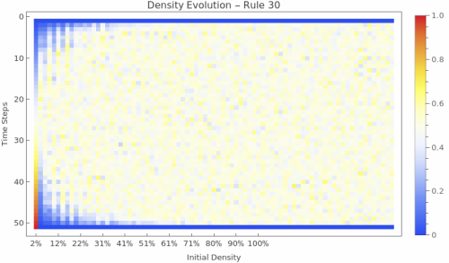
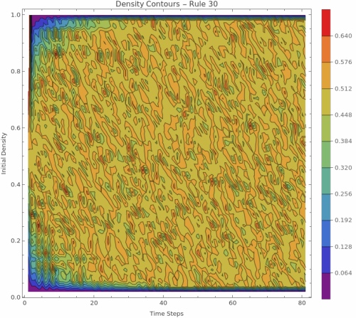
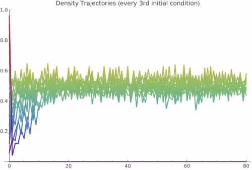
Density Evolution Dynamics: The density evolution heatmap Ï(p,t) shows how density changes over time for ALL possible initial densities simultaneously. Horizontal patterns indicate conservation (density preserved), upward trends show growth dynamics, downward trends indicate decay, and complex curves reveal non-trivial population dynamics. This comprehensive view reveals phase transitions and critical densities.
Conservation vs. Growth Patterns: Horizontal lines in the density evolution indicate conservative rules that maintain density over time. Upward or downward trends show rules that systematically create or destroy cells. Complex curves indicate rules with intricate population dynamics that depend on both initial density and time.
Attractor Analysis: The final density distribution Ï_final(p) reveals the rule's long-term attractors. A diagonal line indicates identity mapping (final density equals initial density), horizontal lines show fixed-point attractors regardless of initial conditions, and complex curves indicate multiple attractors or chaotic behavior with sensitive dependence on initial density.
Critical Phenomena Detection: Sharp transitions in the density evolution heatmap often indicate critical phenomena and phase boundaries. These appear as sudden changes in behavior at specific initial densities, revealing critical thresholds where the rule's qualitative behavior changes dramatically.
Sensitivity Assessment: Smooth gradients in the heatmap indicate robust behavior where small changes in initial density lead to small changes in evolution. Sharp boundaries or chaotic patterns reveal sensitive dependence on initial conditions - the hallmark of chaotic dynamics.
Basin Structure: The final density plot reveals basin structure - regions of initial densities that lead to similar final states. Single attractors appear as horizontal lines, multiple basins show up as plateaus at different levels, and chaotic behavior produces complex, irregular curves.
Research Applications: Use density evolution analysis to classify rules by their population dynamics, identify critical densities and phase transitions, predict long-term behavior from initial conditions, compare different rules quantitatively, and validate theoretical predictions about cellular automaton attractors and conservation laws.
Finite Size Properties
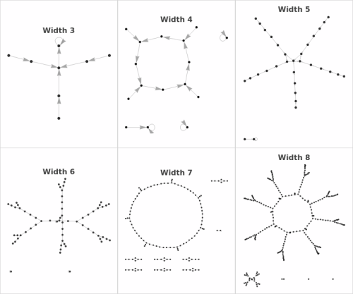
These analyses examine the rule's behavior in small, finite systems, revealing attractor structure and repetition periods. State Transition Diagrams are directed graphs, where each node represents a possible binary configuration of the grid (with periodic boundaries). An arrow connects one state to its successor, given the automaton's rule. Loops and cycles correspond to repeating patternsâattractors in the finite CA. How Would You Construct One by Hand? Choose a grid width (e.g., 3 cells). List all possible states. For 3 cells: 000, 001, 010, 011, 100, 101, 110, 111. For each state: Apply the CA rule (with periodic boundaries) to generate the next state. Cells update according to the values of themselves and their left/right neighbors (use the rule's lookup table). Draw an arrow from the current state to its next state. Repeat until every state is mapped. Visualize the graph: Arrange nodes so cycles (loops) and branches are clear.
State Transition Diagrams
Understanding State Transition Diagrams
State transition diagrams provide a complete map of the cellular automaton's behavior in finite systems, showing every possible configuration and how it evolves. Each node represents a unique binary configuration of the grid (with periodic boundaries), and directed edges show which state follows which under one application of the rule.
Reading the Graphs: In these directed graphs, nodes are numbered 0 to 2^n-1, representing all possible binary strings of length n. An arrow from node A to node B means configuration A evolves to configuration B in one time step. Loops (cycles) indicate repeating patterns - attractors the system settles into. Trees branching into loops show transient states that eventually reach attractors but aren't part of the cycle themselves.
Manual Construction: To construct a state transition diagram by hand: (1) Choose a grid width (e.g., 3 cells). (2) List all possible states (for 3 cells: 000, 001, 010, 011, 100, 101, 110, 111). (3) For each state, apply the CA rule with periodic boundaries - each cell updates based on itself and its left/right neighbors using the rule's lookup table. (4) Draw an arrow from each current state to its successor. (5) Arrange nodes so cycles and branches are visually clear.
Attractor Topology: The graph structure immediately reveals the rule's attractor landscape. Fixed points appear as self-loops (nodes with arrows to themselves). Periodic orbits appear as polygons - triangles for period-3, squares for period-4, etc. Complex rules show intricate branching structures with multiple separate attractor basins, while simple rules often collapse to one or two fixed points.
Transient vs. Recurrent States: States on cycles are recurrent - the system returns to them infinitely often. States not on cycles are transient - visited at most once before reaching an attractor. The ratio of transient to recurrent states indicates how much 'memory' the rule has about initial conditions versus how quickly it forgets and settles into repetitive behavior.
Reversibility Detection: A reversible rule has every node with exactly one incoming edge - each state has exactly one predecessor. This creates a graph of pure cycles with no trees. Non-reversible rules have states with multiple predecessors (many-to-one mapping) and states with no predecessors (Garden of Eden configurations). The visual topology immediately reveals reversibility.
Scale Dependence: As width increases from 3 to 8 cells, watch how complexity grows. Some rules maintain similar simple structures at all scales (suggesting regular, predictable behavior), while others explode into intricate webs of long cycles and complex branching (indicating chaotic or computationally complex dynamics). The scaling behavior is diagnostic of rule class.
Connectivity and Components: The number of disconnected components (separate subgraphs) reveals how many independent attractor basins exist. A single component means all initial conditions eventually interact or merge into one attractor system. Multiple components indicate the rule partitions state space into isolated dynamical subsystems that never influence each other.
Cycle Lengths and Periods: The perimeter of each polygon gives the cycle length. Count the nodes in a loop to determine the period. The longest cycle in the graph is the maximum repetition period for that system size. Comparing maximum cycle lengths across different widths reveals how the rule's temporal complexity scales with spatial size.
Symmetry and Structure: Look for symmetries in the graph layout - they often reflect symmetries in the rule itself (left-right symmetry, complement symmetry, etc.). Highly regular, symmetric graphs suggest simple, structured rules. Asymmetric, irregular graphs indicate complex, less predictable behavior.
Information Flow: The direction of arrows shows information flow through state space. Rules with all short paths to attractors rapidly lose information about initial conditions. Rules with long transient chains preserve initial condition information longer before settling into repetitive behavior.
Research Applications: Use state transition diagrams to classify rules by attractor topology, identify reversible rules visually, count Garden of Eden states, measure basin sizes for different attractors, validate theoretical predictions about finite CA behavior, and understand the complete finite-state dynamics that infinite systems approximate.
Maximum Cycle Length Analysis
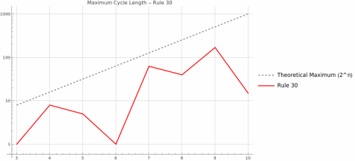
Understanding Cycle Length and Finite Size Properties
Finite size analysis reveals the rule's fundamental mathematical structure by examining complete state spaces in small systems. Since every finite CA must eventually return to a previously visited state, all trajectories lead to attractors - either fixed points (cycle length 1) or periodic cycles. The maximum cycle length provides a measure of the rule's dynamical complexity and computational depth in finite systems.
State Transition Structure: The directed graphs show every possible state and its successor, revealing the rule's complete attractor structure. Cycles appear as polygons (closed loops), while transient states form trees leading to attractors. This topology reveals whether the rule has simple fixed points, complex cycles, or chaotic attractors in finite systems.
Theoretical Maximum and Complexity Bounds: In a system with n cells, there are exactly 2^n possible configurations, providing an absolute upper bound on cycle length. Rules approaching this maximum exhibit highly complex, pseudo-chaotic behavior where the system takes exponentially long to repeat. The ratio of actual maximum cycle to theoretical maximum quantifies the rule's effective state space utilization.
Exponential vs Polynomial Growth: Different rule classes show characteristic scaling behaviors. Class I rules typically maintain cycle length 1 across all system sizes. Class II rules often show small constant or slowly growing cycle lengths. Class III rules may show exponential growth approaching theoretical limits, while Class IV rules can exhibit intermediate polynomial growth patterns.
Reversibility and Cycle Structure: Reversible cellular automata have special properties - every state has exactly one predecessor, so the state space forms disjoint cycles with no transient trees. The cycle length distribution partitions the entire state space into periodic orbits.
Garden of Eden States: States with no predecessors are Garden of Eden configurations. Rules with maximum cycle equal to 2^n have no Garden of Eden states and are necessarily surjective.
Information Theory: Long cycle lengths correspond to high entropy production. The system must remember extensive information about its initial state to know when to return to it, connecting to Kolmogorov-Sinai entropy.
Practical Applications: For cryptography, rules with exponentially growing cycles are desirable. For modeling periodic phenomena, rules with predictable small cycles are useful. For random number generation, rules with maximal cycles provide good pseudo-randomness with known periodicity.
Backtracking Trees
This shows the tree of all possible predecessor configurations that can produce a given target pattern, revealing the rule's preimage structure:

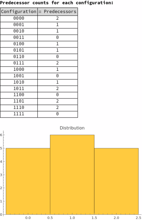
Understanding Backtracking Trees
Backtracking trees reveal the inverse dynamics of cellular automata by showing all possible configurations that could have produced a given target pattern. Unlike forward evolution which is deterministic (one input produces one output), backward evolution is typically non-deterministic - multiple different predecessors can produce the same successor configuration.
Reading the Tree Structure: The root node (top or center) shows the target configuration you're working backward from. Each branch downward represents one time step backward in evolution. At each level, nodes show all possible predecessor configurations. The branching factor indicates how many different ways that configuration could have been produced. Dead ends (leaves) occur when no valid predecessors exist.
Surjectivity and Preimage Structure: The tree immediately reveals whether the rule is surjective (onto). If every possible configuration appears somewhere in the tree when run long enough, the rule is surjective - all configurations are reachable. Configurations that never appear are Garden of Eden states - they have no predecessors and can only exist as initial conditions, never arising from evolution.
Reversibility Detection: A reversible rule produces trees where every node has exactly one child at each level - no branching, just a single path backward. This one-to-one correspondence between successors and predecessors defines reversibility. Non-reversible rules show branching (many-to-one mapping) or dead ends (states with no predecessors).
Expansion vs. Contraction: Watch how the tree grows or shrinks with depth. Expanding trees (branching factor > 1) indicate many configurations map to few - information is being compressed in forward evolution. Contracting trees suggest divergent forward dynamics. Balanced trees indicate conservation of information. The average branching factor quantifies this expansion/contraction rate.
Computational Complexity: The tree's size and structure reveal computational properties. Exponentially growing trees indicate the rule is computationally complex backward - finding predecessors is hard even if forward evolution is simple. Small, finite trees suggest limited backward complexity. The tree's depth and breadth relate to the rule's descriptive complexity.
Pattern Propagation Backward: The tree shows how localized patterns in the target decompose into potentially more complex predecessor patterns. Some rules maintain locality (local patterns have local predecessors), while others show that simple local patterns require complex non-local predecessor arrangements. This reveals the rule's information structure.
Symmetry and Structure: Look for symmetries in the tree - they reflect symmetries in the rule itself. Symmetric trees suggest the rule treats space uniformly. Asymmetric trees may indicate directional bias or broken symmetries. Regular, repetitive tree structure indicates predictable preimage patterns.
Multiple Paths to Same Configuration: If the same configuration appears at multiple positions in the tree at the same depth, it means there are multiple distinct ways to evolve backward to reach that configuration - multiple evolutionary paths converge to the same target. This is diagnostic of information loss in forward evolution.
Depth and Reachability: The maximum depth before the tree terminates (no more valid predecessors exist) indicates how far back you can trace the evolutionary history. Infinite depth suggests all configurations can eventually reach the target through some evolutionary path. Finite depth indicates the target is only reachable from a limited set of initial configurations.
Garden of Eden Identification: Configurations that appear as leaves in deep backtracking trees but never as interior nodes are likely Garden of Eden states - they can serve as predecessors but themselves have no predecessors. Systematically exploring these trees can enumerate all Garden of Eden states for small system sizes.
Information Theory Connection: The branching structure directly relates to information entropy. High branching means forward evolution destroys information (many inputs map to one output). No branching (reversible) means perfect information preservation. The entropy difference between levels quantifies information loss rate.
Comparison Across Rules: Different rule classes show characteristic tree structures. Class I rules often have highly contracting trees (most configurations quickly lead to uniform states). Class II rules show regular, periodic tree structures. Class III rules may have complex, irregular trees. Class IV rules often show intricate, varied branching patterns.
Research Applications: Use backtracking trees to classify rules by preimage structure, identify Garden of Eden states, measure surjectivity, detect reversibility, quantify information loss in forward evolution, understand pattern formation constraints, and study the inverse problem of cellular automaton dynamics.
State Space as Cantor Set
The CA rule as a continuous mapping on [0,1]. Each point represents a binary configuration normalized to the unit interval:
Cantor Set Mapping
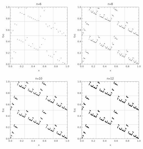
High Resolution View
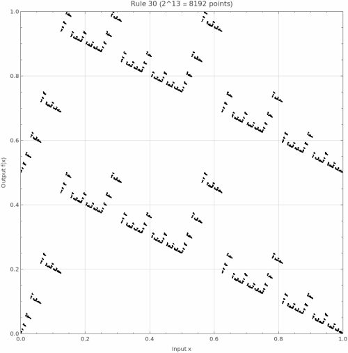
Understanding the Cantor Set Representation
The Cantor set visualization reveals one of the most profound connections between cellular automata and pure mathematics, showing how discrete, local rules generate continuous dynamical systems with rich topological structure. This representation transforms our understanding of CAs from computational objects to mathematical functions with deep geometric properties:
Mathematical Foundation and Construction: Each configuration of n cells can be uniquely encoded as a binary number between 0 and 2^n-1. Dividing by 2^n maps this integer to a point in [0,1]. For example, with n=3, the configuration 101 becomes 5/8 = 0.625. The CA rule then defines a function f:[0,1]â[0,1] where f maps each normalized configuration to its successor. As nââ, the domain converges to a Cantor set - a perfect, nowhere dense, uncountable fractal subset of [0,1] with total length zero but cardinality 2^âµâ.
Continuity from Locality: The CA rule's locality (each cell depends only on its neighborhood) directly implies the function's continuity. Configurations differing by a single bit in position i differ by approximately 1/2^i in the normalized representation. Since the rule's output at any position depends only on nearby bits, small changes in input produce small changes in output. This topological property connects discrete computation to continuous dynamics.
Fractal Self-Similarity and Scaling: The self-similar patterns visible in the plot reflect the rule's shift-invariance and local nature. When you zoom into any region, you see similar structures at finer scales. This isn't just visual aesthetics - it's a fundamental property of the mapping. The fractal dimension of the graph can characterize the rule's complexity, with simple rules producing low-dimensional graphs and complex rules generating space-filling or high-dimensional structures.
Fixed Points and Diagonal Structure: Points on the diagonal y=x represent configurations that don't change under one application of the rule - fixed points in the dynamical system. Periodic orbits appear as discrete sets of points that cycle through each other. The distance from the diagonal indicates how dramatically the rule transforms each configuration. Rules hugging the diagonal are nearly identity functions, while those with large deviations show strong transformative behavior.
Surjectivity and Image Structure: A surjective (onto) rule produces a graph that covers the full unit square, meaning every configuration is reachable from some predecessor. Gaps in the vertical direction reveal non-surjectivity - certain configurations (Garden of Eden states) have no predecessors. The distribution of these gaps provides deep information about the rule's information-theoretic properties and entropy production.
Symbolic Dynamics Connection: This representation directly connects CAs to symbolic dynamics, a branch of dynamical systems theory studying shift spaces. The shift map (moving a configuration one position) becomes conjugate to a topological operation on the Cantor set. Properties like mixing, minimality, and topological entropy have precise meanings in this framework, allowing rigorous analysis of CA behavior using powerful mathematical tools.
Chaos and Sensitivity: In this representation, chaotic behavior manifests as sensitive dependence on initial conditions - nearby input points can map to distant output points. The Lyapunov exponent, measuring exponential separation of trajectories, can be visualized through the local slope of the mapping. Class III rules typically show highly irregular, space-filling graphs indicating chaotic dynamics, while Class I rules produce simple, structured graphs.
Measure Theory and Invariant Measures: For many CA rules, there exists an invariant measure on the Cantor set - a probability distribution preserved by the rule's action. The density of points in different regions of the plot hints at this measure. Rules preserving Bernoulli measure (uniform density) appear as evenly distributed points, while those with non-trivial invariant measures show clustering in specific regions. This connects to ergodic theory and statistical mechanics.
Reversibility and Bijection: Reversible CA rules produce bijective (one-to-one and onto) functions on the Cantor set. In the plot, this appears as a graph where each horizontal line intersects exactly once - every output has exactly one input. The graph of a reversible rule has special symmetry properties and preserves measure, making it a measure-preserving transformation of fundamental importance in ergodic theory.
Computational Complexity from Geometry: The geometric complexity of the Cantor set graph correlates with computational complexity. Simple rules produce smooth or piecewise-linear graphs, while computationally universal rules (like Rule 110) generate graphs with infinite complexity at all scales. The algorithmic information content of the graph's description relates to the rule's computational power.
Research Applications: Use the Cantor set representation to rigorously classify rules by topological properties, compute invariant measures and entropy rates, identify reversible rules through graph symmetry, study bifurcations and phase transitions, connect CA theory to broader dynamical systems theory, and visualize abstract properties like mixing and minimality.